
Resposta rápida
A curva de bomba centrífuga é uma representação gráfica das características de desempenho de uma bomba, plotando altura manométrica, eficiência, consumo de energia e Altura Positiva de Sucção Requerida (NPSHr) em função da vazão. Compreender como ler essa curva é essencial para a seleção correta da bomba, pois o ponto de operação real não é determinado apenas pela bomba, mas pela interseção da curva da bomba com a curva de resistência do sistema. Princípios-chave de seleção:
- A curva H-Q é a principal ferramenta de seleção: Ela mostra quanta altura manométrica (pressão) a bomba gera em cada vazão. A vazão e a altura manométrica requeridas devem se intersectar dentro da Região de Operação Permitida (AOR) da bomba, tipicamente 70–120% da vazão no Ponto de Melhor Eficiência (BEP).
- A curva de eficiência determina o custo operacional: Uma bomba centrífuga opera com máxima eficiência no seu BEP. Operar longe do BEP — abaixo de 50% ou acima de 120% da vazão do BEP — aumenta o consumo de energia, a vibração e o desgaste do selo mecânico.
- A curva de NPSHr é o limite de segurança: O NPSHr aumenta com a vazão. O NPSH disponível (NPSHa) no sistema deve exceder o NPSHr por uma margem mínima — tipicamente 1 metro ou mais — na vazão de operação real, caso contrário a bomba sofrerá cavitação.
- A curva de potência determina o dimensionamento do motor: Para bombas de fluxo radial, o consumo de energia aumenta com a vazão — o motor deve ser dimensionado para a vazão máxima prevista, não apenas para o ponto de projeto.
Uma curva de desempenho de bomba contém as informações-chave que um engenheiro precisa para selecionar, instalar e operar uma bomba centrífuga corretamente. No entanto, a interpretação incorreta dessas curvas é uma das causas mais comuns de erros de seleção de bombas na prática industrial. Uma bomba selecionada apenas pela sua capacidade de atender a uma vazão e altura manométrica de projeto — sem verificar se o ponto de operação está próximo do Ponto de Melhor Eficiência, se a margem de NPSH é adequada em toda a faixa de vazão, ou se a curva do sistema intersecta a curva da bomba em uma região estável — pode operar em cavitação, com alta vibração ou com consumo excessivo de energia por anos antes que o erro subjacente de seleção seja identificado.
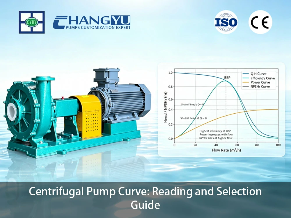
Bombas centrífugas são o tipo de bomba industrial mais amplamente utilizado, e seu desempenho é universalmente comunicado por meio de curvas de bomba padronizadas. Este guia explica cada curva em um gráfico de desempenho de bomba centrífuga, como ler o gráfico para fins de seleção e como evitar os erros mais comuns de interpretação de curvas de bomba.
Quais São as Quatro Curvas-Chave em uma Curva de Desempenho de Bomba Centrífuga?
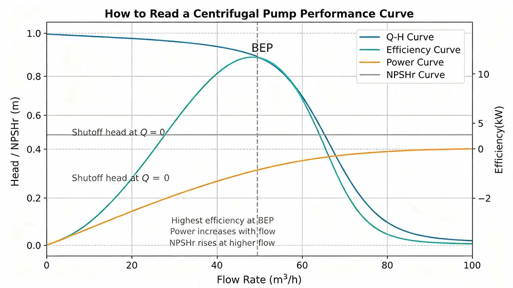
Uma curva de desempenho padrão de bomba centrífuga exibe quatro curvas plotadas em relação a um eixo horizontal comum de vazão (Q). Cada curva fornece informações distintas para a seleção e operação da bomba.
A Curva de Altura Manométrica-Capacidade (H-Q)
A curva H-Q é a base da seleção da bomba. Ela mostra a relação entre a vazão que a bomba entrega e a altura manométrica (pressão) que ela gera. Para uma bomba centrífuga de fluxo radial operando a velocidade constante, a curva H-Q tipicamente inclina-se para baixo da esquerda para a direita — a altura manométrica diminui à medida que a vazão aumenta.
O formato da curva H-Q é determinado pela velocidade específica do rotor. Rotores de baixa velocidade específica (fluxo radial) produzem uma curva relativamente plana. Rotores de alta velocidade específica (fluxo axial) produzem uma curva íngreme, frequentemente com uma característica “depressão” ou formato de sela em baixas vazões. Compreender o formato da curva é importante para a estabilidade de controle — curvas planas são mais sensíveis a pequenas mudanças na resistência do sistema, enquanto curvas íngremes proporcionam controle de vazão mais previsível por meio de estrangulamento.
A Curva de Eficiência (η-Q)
A curva de eficiência mostra a eficiência hidráulica da bomba — a porcentagem da potência de entrada no eixo que é convertida em potência útil do fluido — em toda a faixa de vazão. A curva sobe de zero no fechamento (sem vazão, toda a potência de entrada dissipada como calor), atinge o pico no Ponto de Melhor Eficiência (BEP) e declina em vazões mais altas à medida que as perdas hidráulicas aumentam.
Para fins de seleção, a bomba deve operar dentro de aproximadamente 70–120% da vazão do BEP para aplicações de serviço contínuo. Para serviço intermitente, uma faixa mais ampla pode ser aceitável, mas a operação abaixo de 50% ou acima de 130% da vazão do BEP resultará em desgaste, vibração e custo de energia significativamente aumentados.
Para curvas de bomba com velocidade variável ou múltiplos diâmetros de rotor, linhas de isoeficiência também podem ser exibidas — esses contornos elípticos conectam pontos de igual eficiência em diferentes diâmetros de rotor, ajudando o usuário a identificar a combinação mais eficiente de tamanho de rotor e ponto de operação.
A Curva de Potência (P-Q)
A curva de potência mostra a potência no eixo requerida pela bomba em cada vazão. Para uma bomba padrão de fluxo radial, o consumo de energia aumenta com a vazão — a bomba consome potência mínima no fechamento e potência máxima na extremidade direita da curva. Essa característica tem uma implicação operacional importante: bombas de fluxo radial devem ser iniciadas com a válvula de descarga fechada para minimizar a carga de partida no motor.
Para bombas de fluxo axial, a curva de potência inclina-se para baixo — a potência é máxima no fechamento e diminui à medida que a vazão aumenta. Essas bombas devem ser iniciadas com a válvula de descarga totalmente aberta, caso contrário o motor será sobrecarregado.
A Curva de NPSH Requerido (NPSHr-Q)
A curva de NPSHr mostra a pressão mínima de sucção requerida na entrada da bomba para prevenir cavitação em cada vazão. O NPSHr aumenta com a vazão — à medida que mais fluido passa pelo olho do rotor, a queda de pressão na entrada do rotor aumenta, exigindo maior pressão de sucção para prevenir a formação de bolhas de vapor.
Para operação segura, o NPSH disponível (NPSHa) do sistema deve exceder o NPSHr da bomba por uma margem mínima na vazão de operação real. Uma diretriz comum da indústria é uma margem de pelo menos 1 metro, ou uma razão de NPSHa/NPSHr de 1,1–1,3, o que for maior.
Como Ler uma Curva de Bomba Centrífuga?
Ler uma bomba curva de desempenho é um processo sequencial que extrai informações específicas de cada uma das quatro curvas descritas acima. As etapas a seguir orientam o processo de leitura de uma curva típica de bomba centrífuga de velocidade fixa e diâmetro fixo.
Etapa 1: Localize a vazão necessária no eixo horizontal. A vazão é normalmente indicada em metros cúbicos por hora (m³/h) ou galões por minuto (gpm). Mova-se verticalmente para cima a partir deste ponto.
Etapa 2: Intercepte a curva H-Q. A linha vertical a partir da vazão de projeto interceptará a curva H-Q em um ponto específico. A partir dessa interseção, mova-se horizontalmente para a esquerda para ler a altura manométrica correspondente no eixo vertical. Essa é a altura manométrica que a bomba gerará na vazão de projeto.
Etapa 3: Verifique a eficiência no ponto de operação. A partir do ponto de interseção H-Q, mova-se verticalmente para baixo para interceptar a curva de eficiência. O valor de eficiência nessa vazão determina o custo operacional da bomba. Se a eficiência estiver significativamente abaixo do BEP — por exemplo, mais de 10–15 pontos percentuais abaixo do pico — a bomba pode estar superdimensionada para a aplicação, ou o ponto de operação pode estar muito distante da vazão de projeto da bomba.
Etapa 4: Verifique o consumo de potência. A partir da vazão de projeto, mova-se verticalmente para interceptar a curva de potência. A potência no eixo nessa vazão determina o requisito de tamanho do motor. Para bombas de fluxo radial, verifique se o motor está dimensionado para a vazão máxima possível no sistema — não apenas para a vazão de projeto — para evitar sobrecarga do motor se a bomba operar em vazões superiores às de projeto.
Etapa 5: Verifique a margem de NPSH. A partir da vazão de projeto, mova-se verticalmente para interceptar a curva de NPSHr. Leia o valor de NPSHr. Compare-o com o NPSHa calculado para o sistema. A margem — NPSHa menos NPSHr — deve ser de pelo menos 1 metro na vazão de operação, e preferencialmente maior se a vazão puder aumentar acima do ponto de projeto.
Engenheiros da Changyu Pump observam: Em curvas de bomba simplificadas ou de ponto único, um único valor de NPSHr pode ser fornecido no BEP ou na vazão máxima nominal. No entanto, o NPSHr varia com a vazão e, em curvas de desempenho completas, é plotado como uma curva contínua. Sempre verifique o NPSHr na vazão real de operação — não no final da curva — e garanta margem adequada em toda a faixa de vazão prevista, não apenas no ponto de projeto. Uma bomba que aparenta ter margem de NPSH suficiente na vazão nominal pode cavitar em vazões mais altas se o NPSHa do sistema for marginal.
O Que é o Ponto de Melhor Eficiência (BEP) em uma Curva de Bomba Centrífuga?
O Ponto de Melhor Eficiência (BEP) é a vazão na qual a bomba converte potência no eixo em potência hidráulica com máxima eficiência — o ponto onde as perdas hidráulicas são minimizadas. O BEP é um ponto único na curva H-Q, normalmente marcado por uma linha vertical tracejada ou um rótulo na curva publicada.
Por Que o BEP é Importante
Operar no BEP ou próximo a ele minimiza vários problemas operacionais:
- Vibração: As forças hidráulicas radiais no rotor são equilibradas no BEP. Em vazões significativamente acima ou abaixo do BEP, a distribuição desigual de pressão ao redor do rotor cria cargas radiais desbalanceadas que causam deflexão do eixo e vibração.
- Recirculação na sucção: Em vazões abaixo de aproximadamente 50–60% do BEP, o fluido recircula no olho do rotor, criando padrões de fluxo instáveis, ruído e danos semelhantes à cavitação.
- Elevação de temperatura: Em baixas vazões, uma parcela significativa da potência de entrada é convertida em calor, em vez de trabalho no fluido. Para bombas operando abaixo de 30% da vazão do BEP, o aumento de temperatura na carcaça da bomba pode ser suficiente para causar vaporização do fluido ou danos por expansão térmica.
- Vida útil do selo mecânico e dos rolamentos: As forças desbalanceadas e a vibração que ocorrem fora do BEP reduzem diretamente a vida útil do selo mecânico e dos rolamentos.
Região Operacional Permitida (AOR) e Região Operacional Preferencial (POR)
A AOR é a faixa de vazão dentro da qual a bomba pode operar sem sofrer os graves problemas mecânicos e hidráulicos que ocorrem em condições extremas fora do projeto. A prática da indústria, baseada em normas como ANSI/HI e API 610, normalmente define a AOR como 70–120% da vazão do BEP. Dentro da AOR, a bomba opera com níveis aceitáveis de vibração e estabilidade hidráulica.
A POR é uma faixa mais estreita — normalmente 80–110% da vazão do BEP — dentro da qual a bomba opera com a maior confiabilidade e o menor custo de ciclo de vida. Para bombas críticas e de operação contínua, recomenda-se a especificação dentro da POR.
Saiba mais sobre as curvas de bombas centrífugas abaixo:
Como o Tipo de Rotor Molda a Curva da Bomba Centrífuga?
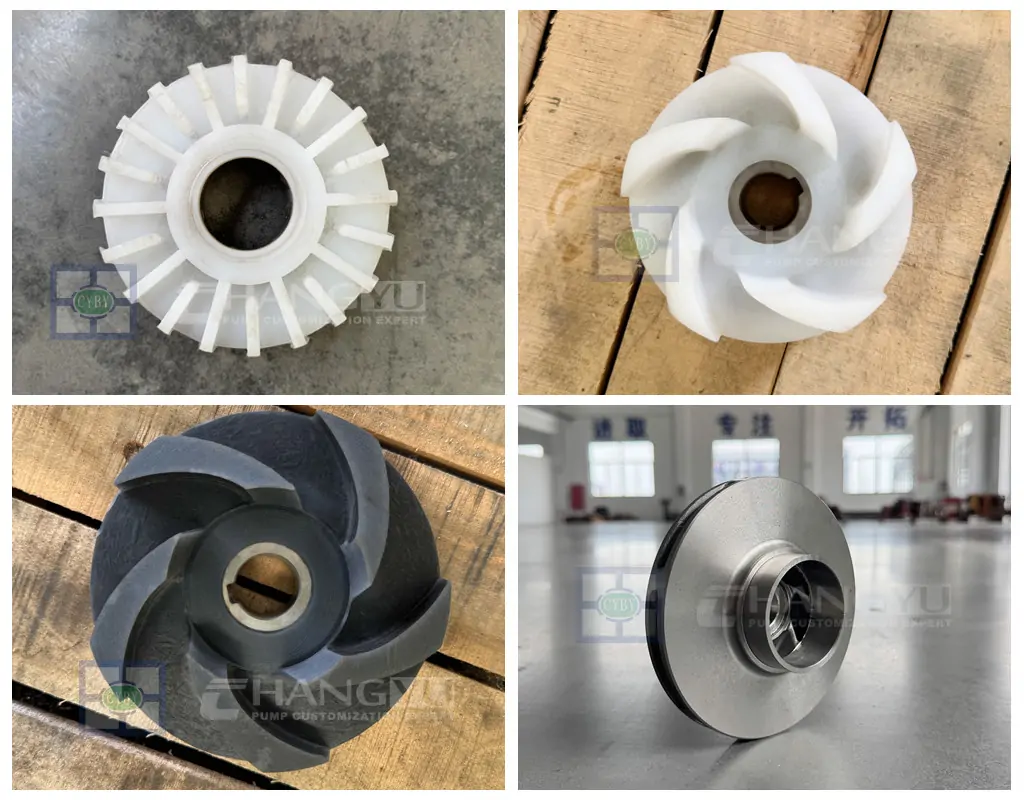
A forma da curva de desempenho de uma bomba centrífuga não é arbitrária — é uma consequência direta da rotação específica (Ns) do rotor, que determina a geometria do rotor e, por meio dela, a relação entre altura manométrica, vazão e potência.
Baixa rotação específica (Ns < 1.500, fluxo radial) : Rotores radiais produzem uma curva H-Q relativamente plana — a altura manométrica muda lentamente conforme a vazão varia. A curva de potência aumenta continuamente com a vazão. Essa combinação significa que bombas de fluxo radial consomem potência mínima no shut-off e podem ser iniciadas com segurança contra uma válvula de descarga fechada. A curva H-Q plana torna essas bombas adequadas para aplicações com requisitos de altura manométrica relativamente constantes, como alimentação de caldeiras e transferência de processo.
Rotação específica média (Ns 1.500–7.000, fluxo misto) : Rotores de fluxo misto produzem uma curva H-Q mais íngreme do que os projetos radiais. A curva de potência é mais plana — o consumo de potência varia de forma menos drástica ao longo da faixa de vazão. Bombas de fluxo misto atendem aplicações de altura manométrica intermediária e alta vazão, como circulação de água de resfriamento e irrigação.
Alta rotação específica (Ns > 7.000, fluxo axial) : Rotores de fluxo axial produzem uma curva H-Q íngreme, frequentemente com uma sela ou queda em baixas vazões. Criticamente, a curva de potência tem inclinação descendente — a potência é máxima no shut-off e diminui com a vazão. Bombas de fluxo axial devem ser iniciadas com a válvula de descarga totalmente aberta para evitar sobrecarga do motor. Essas bombas são usadas em aplicações de altíssima vazão e baixa altura manométrica, como controle de enchentes e elevação de água do mar.
Engenheiros da Changyu Pump enfatizam: Antes de iniciar qualquer bomba centrífuga, verifique a característica da curva de potência. Iniciar uma bomba de fluxo radial com a válvula de descarga aberta, ou uma bomba de fluxo axial com a válvula de descarga fechada, pode sobrecarregar e danificar o motor. Essa verificação simples — confirmada em segundos a partir da curva da bomba — evita uma das causas mais comuns de falha do motor durante a partida.
Para uma explicação detalhada sobre tipos de rotores e classificação de bombas, consulte nosso guia sobre Tipos de Bombas Centrífugas: Um Guia Completo de Classificação.
Como a Velocidade Afeta a Curva da Bomba Centrífuga?
As curvas das bombas são publicadas para uma velocidade de operação específica — normalmente 1.450, 1.750, 2.900 ou 3.500 r/min para bombas acionadas por motor elétrico. Quando a velocidade muda, toda a curva de desempenho se desloca de acordo com as leis de afinidade:
- A vazão (Q) é proporcional à velocidade: Q₂ = Q₁ × (N₂/N₁)
- A altura manométrica (H) é proporcional ao quadrado da velocidade: H₂ = H₁ × (N₂/N₁)²
- A potência (P) é proporcional ao cubo da velocidade: P₂ = P₁ × (N₂/N₁)³
Essas relações assumem similaridade hidráulica — a eficiência permanece aproximadamente constante para variações de velocidade dentro de ±20–30%. Para reduções maiores de velocidade, a eficiência se degrada e as leis de afinidade se tornam menos precisas, exigindo dados de desempenho fornecidos pelo fabricante para uma previsão precisa.
Na prática, os fabricantes de bombas frequentemente publicam múltiplas curvas no mesmo gráfico — cada curva correspondendo a uma velocidade de operação ou diâmetro de rotor diferente — eliminando a necessidade de cálculos manuais das leis de afinidade.
Quando inversores de frequência (VFDs) são usados para controlar a velocidade da bomba, o ponto de operação se move ao longo da curva do sistema conforme a velocidade muda. A bomba permanece próxima do seu BEP em uma faixa de vazões se a curva do sistema for predominantemente de altura manométrica dinâmica (atrito). Se a curva do sistema for predominantemente de altura manométrica estática, o controle por VFD é menos eficaz para manter a eficiência, e métodos alternativos de controle de vazão podem ser mais apropriados.
Como Corresponder a Curva da Bomba Centrífuga à Curva do Seu Sistema para uma Seleção Correta?
A curva da bomba sozinha não determina o ponto de operação da bomba. O ponto de operação é a interseção da curva da bomba com a curva do sistema — um gráfico da altura manométrica total necessária para mover o fluido através do sistema de tubulação em cada vazão.
A Curva do Sistema
Uma curva do sistema tem dois componentes:
- Altura manométrica estática: A elevação vertical do nível do fluido de alimentação até o ponto de descarga, mais qualquer diferença de pressão entre os vasos de alimentação e descarga. A altura manométrica estática é constante, independentemente da vazão.
- Altura manométrica dinâmica: As perdas por atrito em tubulações, válvulas e conexões. A altura manométrica dinâmica aumenta aproximadamente com o quadrado da vazão — a curva é parabólica, subindo de zero na vazão zero.
A curva total do sistema é a soma da altura manométrica estática e da altura manométrica dinâmica em cada vazão.
O Ponto de Operação
A curva da bomba (H-Q) e a curva do sistema se intersectam em um único ponto — o ponto de operação. Nessa vazão, a altura manométrica gerada pela bomba corresponde exatamente à altura manométrica exigida pelo sistema. A bomba operará nesse ponto — não no BEP, não na vazão de projeto, mas na interseção — a menos que a resistência do sistema ou a velocidade da bomba seja alterada.
Para uma seleção correta, a interseção da curva da bomba e da curva do sistema deve cair dentro da AOR da bomba, o mais próximo possível do BEP na prática. Se a interseção cair fora da AOR, a bomba está superdimensionada ou subdimensionada para a aplicação, e uma bomba diferente deve ser selecionada.
Engenheiros da Changyu Pump recomendam: Ao selecionar uma bomba, adicione uma margem de 10–15% à altura manométrica calculada do sistema para considerar o envelhecimento da tubulação, incrustações e incertezas no cálculo hidráulico. No entanto, evite conservadorismo excessivo — uma bomba superdimensionada opera bem à esquerda do BEP, em uma região ineficiente e de alta vibração. Se a margem empurrar o ponto de operação para abaixo de 70% da vazão do BEP, selecione o próximo tamanho menor de bomba e aceite uma altura manométrica de projeto ligeiramente maior.
Estudo de Caso: Como a Leitura Incorreta da Curva de NPSH Causou Danos por Cavitação
Uma estação de tratamento de água municipal operava uma bomba centrífuga horizontal de estágio único e dupla sucção para transferência de água filtrada. A bomba tinha um NPSHr de 4 metros na sua vazão nominal de 500 m³/h. O NPSHa do sistema, calculado durante o projeto original, era de 6 metros — proporcionando uma margem de 2 metros considerada adequada.
Dentro de seis meses após a comissionamento, os operadores da planta relataram níveis crescentes de vibração e um ruído característico de “cascalho” vindo da bomba. As leituras de vibração no alojamento do mancal da bomba aumentaram de 2 mm/s no comissionamento para mais de 12 mm/s. Quando a bomba foi aberta para inspeção, o rotor apresentou danos característicos de cavitação — corrosão por pites e erosão em forma de favo de mel no lado de sucção das pás do rotor.
A investigação da causa raiz revelou que o filtro de sucção estava parcialmente obstruído com detritos, combinado com uma leve queda no nível do tanque de abastecimento durante períodos de pico de demanda. Esses fatores juntos reduziram o NPSHa efetivo dos 6 metros projetados para aproximadamente 2,5 metros — bem abaixo do NPSHr da bomba de 4 metros na vazão de operação. A bomba estava operando em cavitação por vários meses. Os operadores da planta, não familiarizados com a curva da bomba, não entenderam que a vibração crescente era um sintoma de cavitação, e não um problema de mancal.
A equipe de serviço da Changyu Pump limpou o filtro de sucção e ajustou o ponto de ajuste mínimo do nível do tanque de abastecimento, restaurando o NPSHa ao seu valor de projeto. Um sensor de pressão com alarme de baixo NPSH foi instalado na sucção da bomba para fornecer aviso prévio de futuras condições de cavitação. Os operadores foram treinados para ler a curva de NPSHr na vazão real de operação — não na vazão máxima nominal da bomba — e para verificar se o NPSHa do sistema mantinha margem adequada sob todas as condições de operação.
Os níveis de vibração retornaram a 2 mm/s após a correção. O rotor foi substituído durante uma parada programada de manutenção. Nenhum dano adicional por cavitação ocorreu nos três anos seguintes de operação.
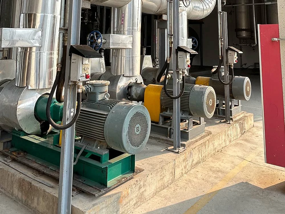
Conclusão principal: A margem de NPSH deve ser verificada na vazão real de operação, não na vazão de projeto ou na vazão máxima nominal da bomba. Um filtro de sucção parcialmente obstruído, uma redução no nível do tanque de abastecimento ou operação em uma vazão maior que a de projeto podem todos reduzir o NPSHa abaixo do NPSHr da bomba. Entender a curva de NPSHr — e monitorar a margem de NPSH ao longo da vida operacional da bomba — previne os danos insidiosos que cavitação causa.
Selecionar a bomba centrífuga correta exige mais do que combinar uma vazão e altura manométrica de projeto. O ponto de operação deve estar dentro da faixa de operação permitida, a margem de NPSH deve ser adequada, e a curva de potência deve ser compatível com o motor e o método de partida. Sempre que possível, selecione uma bomba cujo ponto de melhor eficiência esteja próximo ao ponto de operação normal. Verifique a curva do sistema — não apenas o ponto de projeto — e considere o envelhecimento da tubulação, incrustações e futuras mudanças de serviço. Uma curva de bomba não é uma folha de especificações; é um mapa de desempenho. Lê-la corretamente é a diferença entre uma bomba que opera de forma confiável por anos e uma que causa problemas desde o primeiro dia de operação.
Perguntas Frequentes sobre Curvas de Bombas Centrífugas
P: Quais são as quatro curvas principais em um gráfico de desempenho de bomba centrífuga?
R: A curva de altura manométrica versus vazão (H-Q) mostra a saída de pressão da bomba; a curva de eficiência mostra a eficiência hidráulica; a curva de potência mostra o consumo de potência no eixo; e a curva de NPSHr mostra a pressão mínima de sucção necessária para evitar cavitação.
P: Como encontro o ponto de operação de uma bomba?
R: O ponto de operação é a interseção da curva H-Q da bomba com a curva do sistema. A bomba operará nessa interseção, que pode diferir da vazão de projeto se a resistência real do sistema diferir do cálculo de projeto.
P: O que acontece se uma bomba operar longe do seu Ponto de Melhor Eficiência?
R: A operação abaixo de 50% ou acima de 120% do BEP causa aumento de vibração, cargas radiais desbalanceadas, redução da vida útil de selos e rolamentos e, em vazões muito baixas, aumento de temperatura potencialmente danoso na carcaça da bomba.
P: Por que a curva de NPSHr se inclina para cima?
R: O NPSHr aumenta com a vazão porque taxas de fluxo mais altas criam velocidades de fluido maiores no olho do rotor, o que gera pressões locais mais baixas. É necessária mais pressão de sucção para evitar cavitação em vazões mais altas.
P: Como a alteração da velocidade da bomba afeta a curva de desempenho?
R: De acordo com as leis de afinidade, a vazão muda proporcionalmente com a velocidade, a altura manométrica muda com o quadrado da velocidade e a potência muda com o cubo da velocidade. Essas relações são mais precisas para variações de velocidade dentro de ±20–30%. Para reduções maiores de velocidade, a eficiência se degrada e os dados do fabricante devem ser consultados.
P: Uma bomba centrífuga deve ser iniciada com a válvula de descarga aberta ou fechada?
R: Para bombas de fluxo radial, inicie contra uma válvula de descarga fechada para minimizar a carga de partida. Para bombas de fluxo axial, inicie com a válvula totalmente aberta para evitar sobrecarga do motor. Sempre verifique a característica de potência da curva da bomba antes de iniciar.
Lista de verificação de prevenção do engenheiro de bombas da Changyu
- Leia o NPSHr na vazão operacional real — não no final da curva. O NPSHr aumenta com a vazão, e uma bomba que parece ter margem adequada na vazão de projeto pode cavitar em vazões mais altas se o NPSHa for marginal. Em curvas simplificadas, um único valor de NPSHr pode ser mostrado — verifique se isso se aplica ao seu ponto de operação.
- Trace a curva do sistema contra a curva da bomba antes de finalizar a seleção. O ponto de operação é a interseção dessas duas curvas — não a vazão de projeto. Se a interseção cair fora da AOR, a bomba não terá o desempenho esperado.
- Verifique a característica da curva de potência antes de iniciar qualquer bomba centrífuga. Bombas de fluxo radial (potência aumenta com a vazão) iniciam com a válvula fechada. Bombas de fluxo axial (potência diminui com a vazão) iniciam com a válvula totalmente aberta. Bombas de fluxo misto podem ter uma curva de potência mais plana — consulte o fabricante.
- Adicione uma margem de 10–15% à altura manométrica calculada do sistema — mas evite superdimensionamento excessivo. Uma bomba superdimensionada opera bem à esquerda do BEP, causando vibração e perda de eficiência. Se a margem empurrar o ponto de operação para abaixo de 70% do BEP, selecione a próxima bomba menor.
- Verifique se o motor está dimensionado para a vazão máxima possível, não apenas para a vazão de projeto. Para bombas de fluxo radial, a potência aumenta com a vazão. Se a bomba puder operar em vazões acima das de projeto (por exemplo, durante a partida ou retrolavagem de filtros), o motor deve ser dimensionado para essa condição.
- Monitore a margem de NPSH ao longo da vida operacional da bomba. Entupimento do filtro de sucção, mudanças no nível do tanque de alimentação e aumentos de vazão reduzem o NPSHa. Uma bomba corretamente especificada na comissionamento pode cavitar anos depois se as condições de sucção se degradarem.
- Não opere uma bomba abaixo de 30% da vazão do BEP por períodos prolongados. O aumento de temperatura na carcaça da bomba pode causar vaporização do fluido e danos mecânicos. Um desvio de vazão mínima deve ser instalado para bombas que precisam operar em vazões muito baixas.
- Aplique as leis de afinidade com cautela para grandes mudanças de velocidade. Para aplicações com VFD e reduções de velocidade além de 30%, solicite dados de desempenho fornecidos pelo fabricante em vez de confiar apenas nos cálculos das leis de afinidade.
Conclusão
A curva de uma bomba centrífuga é um documento de engenharia abrangente que comunica o desempenho hidráulico da bomba, eficiência, requisito de potência e limites de cavitação em um formato gráfico padronizado. A interpretação correta das quatro curvas principais — H-Q, eficiência, potência e NPSHr — permite ao usuário verificar se a bomba operará dentro da sua Região Operacional Permitida, próxima ao seu Ponto de Melhor Eficiência, e com margem adequada de NPSH em toda a faixa de vazão prevista. A curva da bomba sozinha, no entanto, não determina o ponto de operação. A curva do sistema — a resistência hidráulica da tubulação conectada — deve ser plotada contra a curva da bomba para identificar a condição operacional real. A interseção dessas duas curvas, não a vazão de projeto na folha de especificações, é onde a bomba operará.
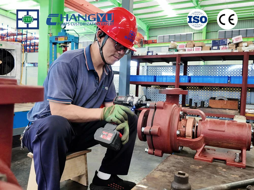
A equipe de engenharia da Changyu Pump oferece suporte de interpretação de curvas de bombas, cálculo de curvas de sistema e seleção de bombas, respaldado por mais de 20 anos de experiência em fabricação de bombas centrífugas em todo o espectro de aplicações industriais.